Tutorial: Graph perturbations with Cellina#
Cellina is a dual-encoder variational autoencoder that separates a cell’s intrinsic state (its identity, \(z\)) from its spatial context (the influence of its neighbours, \(s\)). Because the two are disentangled, we can hold a cell’s identity fixed and ask counterfactual questions about its neighbourhood — a class of queries we call tissue-graph counterfactuals.
In this notebook we:
Load and pre-process a colorectal cancer (CRC) spatial dataset [CRH+25]
Train
CellinaVisualise the two latent spaces (\(z\), \(s\)) to confirm the disentanglement
Run two types of counterfactual interventions (as in silico graph perturbations) on a held-out cancer cell population:
Edge perturbation — rewire a cell’s neighbourhood
Node perturbation — alter the expression of its neighbours
%matplotlib inline
%reload_ext autoreload
%autoreload 2
import numpy as np
import scanpy as sc
import torch
import os
import matplotlib.pyplot as plt

from sklearn.model_selection import train_test_split
from scvi.train._callbacks import SaveCheckpoint, EarlyStopping
from scipy.stats import pearsonr

from cellina import Cellina, make_neighbor_perturbation
from cellina._spatial_utils import spatial_neighbors, compute_spatial_features
# Fixing seeds and ensuring deterministic behavior for reproducibility
seed = 0
np.random.seed(seed)  # NumPy
torch.manual_seed(seed)  # PyTorch CPU
torch.cuda.manual_seed(seed)  # PyTorch GPU (single-GPU)
torch.backends.cudnn.deterministic = True
torch.backends.cudnn.benchmark = False
1. Data preprocessing#
We use scanpy [WAT18] for loading, QC, normalisation, and the UMAP visualisations below.
Load adata and preprocess#
adata = sc.read(
    f"./data/crc_232.h5ad",
    backup_url=f"https://zenodo.org/records/15574384/files/232.h5ad?download=1"
)
adata.obs_names_make_unique()
For the CRC data, we define a custom celltype label map which groups together major cell types - needed as e.g. epi1-4 correspond to different epithelial subtypes found in healthy and diseased tissues.
label_to_coarse = {
    "epi1": "Epithelial",
    "epi2": "Epithelial",
    "epi3": "Epithelial",
    "epi4": "Epithelial",

    "fib1": "Fibroblast",
    "fib2": "Fibroblast",

    "EC": "Endothelial",
    "SMC": "Smooth_muscle",

    "BC": "B_cell",
    "PC_IgA": "Plasma_cell",
    "PC_IgG": "Plasma_cell",
    "PC_IgM": "Plasma_cell",

    "TC": "T_cell",

    "mye1": "Myeloid",
    "mye2": "Myeloid",

    "mast": "Mast_cell",
}

adata.obs["coarse_type"] = adata.obs['ist'].map(label_to_coarse)
# Set annotation keys
labels_key = 'coarse_type'
domains_key = 'typ'
batch_key = None
# Filtering and QC
adata = adata[~adata.obs[domains_key].isna()]
adata = adata[~adata.obs[labels_key].isna()]

sc.pp.filter_cells(adata, min_counts=3)
sc.pp.filter_genes(adata, min_counts=3)
# HVG selection
adata.layers['counts'] = adata.X.copy()
sc.pp.highly_variable_genes(adata, layer='counts', flavor='seurat_v3', n_top_genes=2000, subset=True)
Data splits#
For this demo, we will holdout Myeloid cells in the cancer (CRC) region
holdout_ct = 'Myeloid'
is_tumor_region  = adata.obs[domains_key].str.contains("CRC", regex=True)
is_holdout_ct = adata.obs[labels_key] == holdout_ct

# Combine for test set
test_mask = (is_tumor_region) & (is_holdout_ct)
test_idx = np.where(test_mask)[0]

# Get train/val indices
all_idx = np.arange(adata.n_obs)
trainval_idx = np.setdiff1d(all_idx, test_idx)
adata.obs['is_holdout'] = False
adata.obs.iloc[test_idx, adata.obs.columns.get_loc('is_holdout')] = True
validation_size = 0.1
train_idx, val_idx = train_test_split(
    trainval_idx,
    test_size=validation_size,
    random_state=0,
    shuffle=True,
)
print("Train size:", len(train_idx))
print("Validation size:", len(val_idx))
print("Test size:", len(test_idx))
Train size: 96258
Validation size: 10696
Test size: 5035
Spatial features preprocessing#
As we are performing an out-of-distribution inference on CRC Myeloids, we want to keep them out when computing adjacency and spatial feature aggregation. We store original adjacency structure for inference.
sc.pp.normalize_total(adata, target_sum=1e4)
sc.pp.log1p(adata)

max_neighbors = 200
adata.obsm['spatial'] = adata.obs[['CenterX_global_px', 'CenterY_global_px']].values
adata.obsp['spatial_connectivities_orig'] = spatial_neighbors(adata, bandwidth=100 / 0.12028,
                                                              max_neighbours=max_neighbors,
                                                              standardize=False,
                                                              inplace=False)

# Recompute with test indices masked out, to avoid data leakage in spatial features for test set
spatial_neighbors(adata, bandwidth=100 / 0.12028,
                  max_neighbours=max_neighbors,
                  standardize=False,
                  test_indices=test_idx)
compute_spatial_features(adata)

adata.X = adata.layers['counts'].copy()  # reset to raw counts for cellina
2. Training#
The model in brief#
Cellina is a graph VAE with two latent variables per cell: \(z\) for intrinsic identity and \(s\) for spatial context. We disentangle them to enable counterfactual queries about a cell’s neighbourhood.
Generative model. — a (graph) Variational Autoencoder VAE [KW13] that uses a Negative-Binomial likelihood raw counts — a standard noise model for over-dispersed single-cell count data [LRC+18]. Cellina is implemented on top of scvi-tools [GLX+22], and encodes each cell into two latent variables with standard-normal priors,
where \(z\) captures intrinsic identity (from the cell’s own counts \(x\)) and \(s\) captures spatial context. For the base model, \(\varphi(v) = \big(\sum_{u\in\mathcal{N}(v)} W_{uv}\,\tilde{x}_u\big)\big/\big(\sum_{u\in\mathcal{N}(v)} W_{uv}\big)\) is the degree-normalised aggregation of the (log-normalised) neighbour expression \(\tilde{x}_u\). The decoder reconstructs counts from the concatenation \([z;\,s]\). The library size is treated as observed, so only \(z\) and \(s\) contribute KL terms to \(\mathcal{L}_\mathrm{VAE}\) (the negative ELBO).
Supervised disentanglement. Maximising the ELBO alone does not stop \(z\) from absorbing spatially-driven variation, so Cellina adds two auxiliary objectives on \(z\):
a cell-type classifier (\(\mathcal{L}_\mathrm{clf}\)) anchors \(z\) to cell identity \(y\);
a domain adversary: a discriminator is trained to predict the spatial domain \(d\) from a detached \(z\) (\(\mathcal{L}_\mathrm{disc}\)), and the encoder is then trained to fool it (\(\mathcal{L}_\mathrm{adv}\)), pushing domain information out of \(z\) and (by elimination) into \(s\).
The Cellina-GAT variant additionally applies a graph-supervised contrastive loss \(\mathcal{L}_\mathrm{spatial}\) on \(s\) — a SupCon variant [KTW+20] where a cell’s spatial neighbours are positives and different-domain non-neighbours are negatives — encoding the inductive bias that nearby cells share a microenvironment. The base model has no such term.
Objective: weights (\(\lambda\)) and normalisation (\(\alpha\)). The objective minimised over the encoder/decoder is
The \(\lambda\) are the user-set weights — classifier_lambda, discriminator_lambda, link_prediction_weight below — and all default to \(1\). Because the reconstruction and auxiliary losses live on very different scales, each auxiliary term is also rescaled by a data-adaptive normalisation factor \(\alpha_\bullet = \overline{|\mathcal{L}_\mathrm{VAE}|} \,/\, (\overline{|\mathcal{L}_\bullet|} + \epsilon)\) — a ratio of mean loss magnitudes measured over the first epoch and then frozen. This is switched on with normalize_losses=True in plan_kwargs, and is what makes unit weights a robust default.
Training alternates two steps per batch: (1) update the discriminator on a detached \(z\) (VAE frozen); (2) update the encoder and decoder on \(\mathcal{L}\) above (discriminator frozen) — the standard adversarial (GAN) schedule [GPAM+14].
Related work (in brief). Non-spatial perturbation models — scGen [LWT19], CPA [HBK+22, LKSDD+23], and CellFlow [KFB+25] — predict cellular responses but assume i.i.d. cells and a shared stimulus, ignoring a cell’s spatial neighbourhood. Spatial models instead separate intrinsic from niche-driven variation (e.g. SIMVI [DSK+25]) or perform in silico spatial perturbations (MintFlow [ASJ+25], CONCERT [LKG+25], Celcomen [MCP+25], SpatialProp [SBBZ25]). Cellina enables two types of in silico spatial perturbations (according to the graph counterfactual described above): edge interventions (rewiring a cell’s neighbourhood) and node interventions (altering the expression of its neighbours) — see below.
train_args = {
    "max_epochs": 100,
    "batch_size": 2048,
    "check_val_every_n_epoch": 1,
    "early_stopping": True,
    "enable_checkpointing": True,
    "early_stopping_patience": 10,
    "early_stopping_monitor": "vae_loss_validation",
    "devices": [0],
    "datasplitter_kwargs": {"external_indexing": [train_idx, val_idx, test_idx]},
    "callbacks": [
        SaveCheckpoint(
            monitor='vae_loss_validation',
            dirpath=f"scvi_log/cellina/",
            load_best_on_end=True),
        EarlyStopping(
            monitor="vae_loss_validation",
            patience=10,
            mode="min"),
            ],
}

plan_kwargs = {
    "lr": 1e-3,
    "normalize_losses": True,  # compute the per-loss normalization scales (alpha) over epoch 0
}
We now define the model arguments and train Cellina. The *_lambda weights are the user-set \(\lambda\) from the objective above; we keep them at their unit default.
cellina_args = {
    "n_latent": 64,
    "use_observed_lib_size": True,
    "condition_on_intrinsic": False,
    "classifier_lambda": 1.0,      # lambda_clf  (cell-type classifier on z)
    "discriminator_lambda": 1.0,   # lambda_adv  (domain adversary on z)
    "gene_likelihood": "nb",       # Negative Binomial likelihood
    'n_layers': 2,
}
Cellina.setup_anndata(adata,
                      batch_key=batch_key,
                      labels_key=labels_key,
                      domains_key=domains_key,
                      spatial_obsm_key='spatial_x',
                      layer='counts')
cellina_model = Cellina(adata, **cellina_args)
INFO     Generating sequential column names
INFO     cellina: The Cellina model has been initialized with adversarial domain forgetting
cellina_model.train(**train_args, plan_kwargs=plan_kwargs)
INFO     File
         /data/ddimitrov/repos/cellina/docs/scvi_log/cellina/epoch=32-step=3072-vae_loss_validation=325.77386474609
         375/model.pt already downloaded
Monitored metric vae_loss_validation did not improve in the last 10 records. Best score: 325.774. Signaling Trainer to stop.
Cellina-GAT variant. A second variant,
CellinaGCN(withconvolution_type='gat'), replaces the fixed degree-normalized aggregator \(\varphi(v)\) with GATv2 attention [BAY21] over each cell’s local subgraph. It therefore operates on the spatial graph directly and does not needcompute_spatial_features(skip that preprocessing step and passspatial_connectivities_keytosetup_anndatainstead). It also adds the contrastive loss \(\mathcal{L}_\mathrm{spatial}\) described above, whose weight islink_prediction_weight(\(\lambda_\mathrm{spatial}\), default \(1\)). This notebook focuses on the baseCellinamodel.
3. Qualitative Analysis#
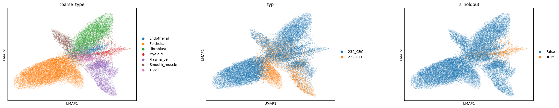
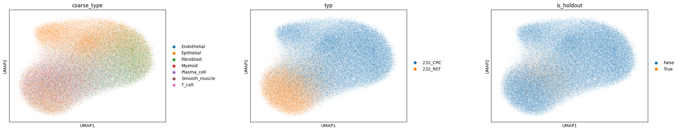
We visualise the two latent spaces. If the disentanglement worked, the intrinsic representation \(z\) should cluster by cell type while being mixed across domains (the adversary removed domain signal), whereas the spatial representation \(s\) should instead organise by tissue region (REF, TVA, CRC).
checkpoint_name = os.listdir("scvi_log/cellina/")[0]
model = Cellina.load(
    f"scvi_log/cellina/{checkpoint_name}",
    adata=adata,
)
INFO     File scvi_log/cellina/epoch=32-step=3072-vae_loss_validation=325.77386474609375/model.pt already
         downloaded
INFO     cellina: The Cellina model has been initialized with adversarial domain forgetting
adata.obsm['cellina_basal'] = model.get_latent_representation(latent_key='z', batch_size=2048)
adata.obsm['cellina_spatial'] = model.get_latent_representation(latent_key='s', batch_size=2048)
sc.pp.neighbors(adata, use_rep='cellina_basal')
sc.tl.umap(adata)
sc.pl.umap(adata, color=[labels_key, domains_key, 'is_holdout'], wspace=0.4)
sc.pp.neighbors(adata, use_rep='cellina_spatial')
sc.tl.umap(adata)
sc.pl.umap(adata, color=[labels_key, domains_key, 'is_holdout'], wspace=0.4)
4. Counterfactuals#
A tissue-graph counterfactual asks: what would a cell express if its neighbourhood context changed, while its intrinsic identity stayed fixed? The spatial graph \(\mathcal{G}\) has two mutable parts — its edges (neighbourhood topology) and its node features (neighbour expression) — giving two perturbation types, both applied post-training:
Edge perturbation modifies a cell’s neighbours \(\mathcal{N}(v)\).
Node perturbation modifies the gene features \(\{x_u : u \in \mathcal{N}(v)\}\) of fixed neighbours.
In both cases we evaluate on the held-out cancer Myeloids: cells whose true tumour-context expression the model never saw during training. We compare the observed healthy→cancer log-fold change (ground truth) against the predicted one (counterfactual).
4.1 Edge perturbation#
Edge perturbation (Definition 1) intervenes on a cell’s neighbourhood, \(\mathcal{N}(v) := \mathcal{N}'\) — neighbours may be added, removed, or replaced.
Here we evaluate it as a domain edge-rewiring. Let \(\mathcal{I}_y\) be the focal cells of type \(y\) (Myeloid) in the source domain (healthy, REF), and let \(\mathcal{P}_{\setminus y}\) be the cells in the target domain (cancer, CRC) observed as neighbours of type-\(y\) cells there — excluding type \(y\) itself, which keeps the counterfactual conservative. For each focal cell \(v \in \mathcal{I}_y\) we sample new neighbours \(\mathcal{N}' \sim \mathcal{P}_{\setminus y}\) and set \(\mathcal{N}(v) := \mathcal{N}'\). Since the cancer Myeloids were held out of the training graph, this tests whether Cellina can predict how a healthy Myeloid would shift if placed in a tumour microenvironment it never saw.
First, we get indices of control and target cells. Control cells are Myeloids that we have seen during training (in the healthy region), and target cells are Myeloids in the cancer region that were held-out during training. We call these target cells because we want to apply in-silico perturbations to control cells to look like target cells.
is_control_region = adata.obs[domains_key].str.contains('REF')
mask_control = is_control_region & is_holdout_ct
idx_control = np.where(mask_control.values)[0]

mask_target = is_tumor_region & is_holdout_ct
idx_target = np.where(mask_target.values)[0]
Now, we want to get the indices of cells from which to sample new neighbouring cells for healthy Myeloids i.e. the set of observed neighbours of cancer Myeloids (\(\mathcal{P}_{\setminus y}\), excluding Myeloids themselves).
# "neighbour_indices" are indices of the neighbors of idx_target cells
conn = adata.obsp["spatial_connectivities_orig"]
sub_conn = conn[idx_target]                # rows for target cells
neighbor_indices = sub_conn.nonzero()[1]   # all neighbors at once
neighbor_indices = np.unique(neighbor_indices)
# remove neighbors having same ct as holdout_ct
neighbor_indices = neighbor_indices[~is_holdout_ct.values[neighbor_indices]]
get_counterfactual_expression rewires each control cell’s neighbourhood by sampling from neighbour_indices and decodes the new expression. (precomputed=False recomputes the aggregated spatial features \(\varphi(v)\) from the sampled neighbours.)
args_gex = {
    "indices": idx_control,
    "batch_size": 2048,
    "seed": 0,
    "neighbour_indices": neighbor_indices,
    "precomputed": False,
}

counterfactual_counts = model.get_counterfactual_expression(**args_gex)
INFO AnnData object appears to be a copy. Attempting to transfer setup.
def _normalize_counts(x, eps=1e-8, scale=1e4):
    return x / (x.sum(axis=1, keepdims=True) + eps) * scale

def safe_log2_fold_change(a, b, eps=1e-6):
    """
    Compute log2((a + eps) / (b + eps)) elementwise.
    Use this instead of log2(a - b). eps should be set relative to normalized scale.
    """
    a = np.asarray(a)
    b = np.asarray(b)
    return np.log2((a + eps) / (b + eps))

def get_lfc(control, target, counterfactual, normalize_counts=True, n_deg=200):
    if normalize_counts:
        control = _normalize_counts(control)
        target = _normalize_counts(target)
        counterfactual = _normalize_counts(counterfactual)

    mean_control = np.nanmean(control, axis=0)
    mean_target = np.nanmean(target, axis=0)
    mean_cf = np.nanmean(counterfactual, axis=0)

    # compute log2 fold changes
    gt_vec = safe_log2_fold_change(mean_target, mean_control)
    cf_vec = safe_log2_fold_change(mean_cf, mean_control)

    deg_scores = np.abs(gt_vec)
    top_features = np.argsort(-deg_scores)[:n_deg]

    return gt_vec, cf_vec, top_features
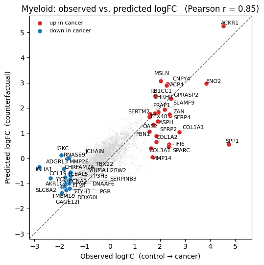
Finally, we compare the ground-truth log-fold change (healthy vs. cancer Myeloids) against the counterfactual one (healthy vs. edge-perturbed Myeloids). We highlight the top differentially-expressed genes (largest \(|\)observed logFC\(|\)) and report Pearson’s \(r\) over them.
control = np.array(adata.layers['counts'][mask_control.values, :].todense())
target = np.array(adata.layers['counts'][mask_target.values, :].todense())
counterfactual = counterfactual_counts

true_lfc, pred_lfc, deg = get_lfc(control=control, target=target, counterfactual=counterfactual, n_deg=50)
pearson, _ = pearsonr(true_lfc[deg], pred_lfc[deg])
As we see, Cellina transforms healthy Myeloid cells into cancer-like Myeloids purely by swapping their neighbours — recovering the observed direction and magnitude of the top gene changes.
from adjustText import adjust_text


def plot_lfc(true_lfc, pred_lfc, deg, gene_names, holdout_ct, pearson):
    """Scatter of observed vs. predicted logFC, highlighting the top DE genes.

    Top genes are coloured by the direction of the *observed* change and their
    names are repelled with adjustText so the labels stay legible.
    """
    fig, ax = plt.subplots(figsize=(6, 5.5))

    deg = np.asarray(deg)
    non_deg = np.setdiff1d(np.arange(len(true_lfc)), deg)

    # background (non-DE) genes
    ax.scatter(true_lfc[non_deg], pred_lfc[non_deg],
               alpha=0.25, s=8, color="lightgray", linewidths=0, rasterized=True)

    # top DE genes, coloured by the direction of the observed change
    up = deg[true_lfc[deg] >= 0]
    down = deg[true_lfc[deg] < 0]
    ax.scatter(true_lfc[up], pred_lfc[up], s=45, color="#d62728",
               edgecolor="white", linewidths=0.5, zorder=3, label="up in cancer")
    ax.scatter(true_lfc[down], pred_lfc[down], s=45, color="#1f77b4",
               edgecolor="white", linewidths=0.5, zorder=3, label="down in cancer")

    # repelled gene labels
    texts = [ax.text(true_lfc[i], pred_lfc[i], gene_names[i], fontsize=8) for i in deg]
    adjust_text(texts, ax=ax, arrowprops=dict(arrowstyle="-", color="0.6", lw=0.5))

    # identity line
    lo = float(min(true_lfc.min(), pred_lfc.min()))
    hi = float(max(true_lfc.max(), pred_lfc.max()))
    pad = 0.05 * (hi - lo)
    lims = [lo - pad, hi + pad]
    ax.plot(lims, lims, "k--", lw=1, alpha=0.6, zorder=1)
    ax.set_xlim(lims)
    ax.set_ylim(lims)
    ax.set_aspect("equal")

    ax.set_xlabel("Observed logFC  (control → cancer)")
    ax.set_ylabel("Predicted logFC  (counterfactual)")
    ax.set_title(f"{holdout_ct}: observed vs. predicted logFC   (Pearson r = {pearson:.2f})")
    ax.legend(frameon=False, fontsize=8, loc="upper left")
    fig.tight_layout()
    plt.show()
gene_names = np.array(adata.var_names)

plot_lfc(true_lfc, pred_lfc, deg, gene_names, holdout_ct, pearson)
4.2 Node perturbation#
Node perturbation (Definition 2) keeps the graph topology fixed but edits the neighbours’ feature vectors. For a target gene set \(\mathcal{S}\),
The transformation \(T_g\) is arbitrary (knockout, overexpression, an additive shift, …); restricting it to a gene set \(\mathcal{S}\) is biologically motivated, since genes act in co-regulated programs (a pathway or regulon). Biologically, this mimics an intervention — e.g. a CRISPR perturbation — applied to the neighbouring cells. Here we instantiate \(T_g\) as the observed healthy→cancer log-fold change of the top-\(n\) genes, estimated per cell type by pseudobulk. Crucially, the held-out Myeloid population is shifted by the global (cell-type-averaged) change rather than its own, so the model never sees the true Myeloid perturbation it is asked to predict.
n_pert_genes = 200 # NOTE: we assume that a smaller number would be approriate for targeted perturbations, while for our cancer case we want to capture a broader phenotypic shift with more genes
control_domain = '232_REF'
target_domain = '232_CRC'
Here we define helper functions to compute the perturbation logFC (global and cell-type-specific) from pseudobulk profiles, using decoupler [BiMVelezSB+22].
import pandas as pd
import scipy.sparse as sp
import decoupler as dc

def get_perturbation_logfc(adata, control_domain, holdout_domain, labels_key, domains_key):
    # Cell-type-specific
    pdata_ct = dc.pp.pseudobulk(
        adata=adata, sample_col=domains_key, groups_col=labels_key, mode='sum', layer='counts'
    )
    sc.pp.normalize_total(pdata_ct, target_sum=1e4)
    sc.pp.log1p(pdata_ct)

    cell_types_with_both = [
        ct for ct in pdata_ct.obs[labels_key].unique()
        if ((pdata_ct.obs[domains_key] == control_domain) & (pdata_ct.obs[labels_key] == ct)).any()
        and ((pdata_ct.obs[domains_key] == holdout_domain) & (pdata_ct.obs[labels_key] == ct)).any()
    ]

    _ct_rows = []
    for _ct in cell_types_with_both:
        _crc_ct = pdata_ct[(pdata_ct.obs[domains_key] == holdout_domain) & (pdata_ct.obs[labels_key] == _ct)].X
        _ref_ct = pdata_ct[(pdata_ct.obs[domains_key] == control_domain) & (pdata_ct.obs[labels_key] == _ct)].X
        _crc_m  = np.asarray(_crc_ct.mean(axis=0)).flatten() if sp.issparse(_crc_ct) else _crc_ct.mean(axis=0).flatten()
        _ref_m  = np.asarray(_ref_ct.mean(axis=0)).flatten() if sp.issparse(_ref_ct) else _ref_ct.mean(axis=0).flatten()
        _ct_rows.append(pd.Series(_crc_m - _ref_m, index=pdata_ct.var_names, name=_ct))
    domain_logfc_df = pd.concat(_ct_rows, axis=1).T

    return domain_logfc_df


def get_global_perturbation_logfc(adata, control_domain, holdout_domain, labels_key, domains_key, holdout_ct):
    adata_sub = adata[adata.obs[labels_key]!=holdout_ct]
    pdata_global = dc.pp.pseudobulk(
        adata=adata_sub, sample_col=domains_key, groups_col=None, mode='sum', layer='counts'
    )
    sc.pp.normalize_total(pdata_global, target_sum=1e4)
    sc.pp.log1p(pdata_global)

    _holdout_X    = pdata_global[pdata_global.obs[domains_key] == holdout_domain].X
    _control_X    = pdata_global[pdata_global.obs[domains_key] == control_domain].X
    _holdout_mean = np.asarray(_holdout_X.mean(axis=0)).flatten() if sp.issparse(_holdout_X) else _holdout_X.mean(axis=0).flatten()
    _control_mean = np.asarray(_control_X.mean(axis=0)).flatten() if sp.issparse(_control_X) else _control_X.mean(axis=0).flatten()

    return pd.Series(_holdout_mean - _control_mean, index=pdata_global.var_names)
# Cell-type-specific perturbation
domain_logfc_df = get_perturbation_logfc(adata, control_domain, target_domain, labels_key, domains_key)
global_logfc_series = get_global_perturbation_logfc(adata, control_domain, target_domain, labels_key, domains_key, holdout_ct)
domain_logfc_df.loc[holdout_ct, global_logfc_series.index] = global_logfc_series # NOTE: set the holdout celltype's perturbation to the global perturbation - ct

logfc_series_dict = {}
for ct in domain_logfc_df.index:
    s = domain_logfc_df.loc[ct]
    top_g = s.abs().nlargest(n_pert_genes).index.tolist()
    logfc_series_dict[ct] = s[top_g]
For base Cellina, the shift is applied additively in log-space on the aggregated neighbour features (make_neighbor_perturbation, add_shift=True), then re-aggregated into the spatial features \(\varphi(v)\) before inference. (For the Cellina-GAT variant, the shift is instead applied to each neighbour cell individually via make_perturbed_expression and a cf_layer, and aggregated by the GAT on the fly.)
adata.X = adata.layers['counts'].copy()
sc.pp.normalize_total(adata, target_sum=1e4)
sc.pp.log1p(adata)

make_neighbor_perturbation(
        adata,
        perturbations=logfc_series_dict,
        groupby=labels_key,
        obsm_key_out='spatial_x_cf',
        base=np.e,
        renormalize=True,
        add_shift=True,
)
pert_expr = model.get_perturbed_expression(
    adata=adata, indices=idx_control, spatial_obsm_key='spatial_x_cf',
    batch_size=2048, library_size=1e4,
)
WARNING: adata.X seems to be already log-transformed.
control = np.array(adata.layers['counts'][mask_control.values, :].todense())
target = np.array(adata.layers['counts'][mask_target.values, :].todense())
counterfactual = pert_expr

true_lfc, pred_lfc, deg = get_lfc(control=control, target=target, counterfactual=counterfactual, n_deg=20)
pearson, _ = pearsonr(true_lfc[deg], pred_lfc[deg])
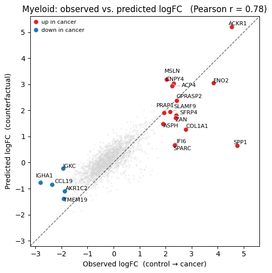
Once again, Cellina predicts the effect of the neighbouring gene modifications on the held-out Myeloid population.
plot_lfc(true_lfc, pred_lfc, deg, gene_names, holdout_ct, pearson)
References#
Amir Akbarnejad, Lloyd Steele, Daniyal J Jafree, Sebastian Birk, Marta Rosa Sallese, Koen Rademaker, Adam Boxall, Benjamin Rumney, Catherine Tudor, Minal Patel, and others. Mapping and reprogramming human tissue microenvironments with mintflow. bioRxiv, 2025.
Pau Badia-i-Mompel, Jesús Vélez Santiago, Jana Braunger, Celina Geiss, Daniel Dimitrov, Sophia Müller-Dott, Petr Taus, Aurelien Dugourd, Christian H Holland, Ricardo O Ramirez Flores, and others. Decoupler: ensemble of computational methods to infer biological activities from omics data. Bioinformatics advances, 2(1):vbac016, 2022.
Shaked Brody, Uri Alon, and Eran Yahav. How attentive are graph attention networks? arXiv preprint arXiv:2105.14491, 2021.
Helena L Crowell, Irene Ruano, Zedong Hu, Yourae Hong, Gin Caratù, Hubert Piessevaux, Ashley Heck, Rachel Liu, Max Walter, Megan Vandenberg, and others. Tracing colorectal malignancy transformation from cell to tissue scale. bioRxiv, 2025.
Mingze Dong, David G Su, Harriet Kluger, Rong Fan, and Yuval Kluger. Simvi disentangles intrinsic and spatial-induced cellular states in spatial omics data. Nature Communications, 16(1):2990, 2025.
Adam Gayoso, Romain Lopez, Galen Xing, Pierre Boyeau, Valeh Valiollah Pour Amiri, Justin Hong, Katherine Wu, Michael Jayasuriya, Edouard Mehlman, Maxime Langevin, and others. A python library for probabilistic analysis of single-cell omics data. Nature biotechnology, 40(2):163–166, 2022.
Ian J Goodfellow, Jean Pouget-Abadie, Mehdi Mirza, Bing Xu, David Warde-Farley, Sherjil Ozair, Aaron Courville, and Yoshua Bengio. Generative adversarial nets. Advances in neural information processing systems, 2014.
Leon Hetzel, Simon Boehm, Niki Kilbertus, Stephan Günnemann, Mohammad Lotfollahi, and Fabian Theis. Predicting cellular responses to novel drug perturbations at a single-cell resolution. In S. Koyejo, S. Mohamed, A. Agarwal, D. Belgrave, K. Cho, and A. Oh, editors, Advances in Neural Information Processing Systems, volume 35, 26711–26722. Curran Associates, Inc., 2022. URL: https://proceedings.neurips.cc/paper_files/paper/2022/file/aa933b5abc1be30baece1d230ec575a7-Paper-Conference.pdf.
Prannay Khosla, Piotr Teterwak, Chen Wang, Aaron Sarna, Yonglong Tian, Phillip Isola, Aaron Maschinot, Ce Liu, and Dilip Krishnan. Supervised contrastive learning. CoRR, 2020. URL: https://arxiv.org/abs/2004.11362, arXiv:2004.11362.
Diederik P Kingma and Max Welling. Auto-encoding variational bayes. arXiv preprint arXiv:1312.6114, 2013.
Dominik Klein, Jonas Simon Fleck, Daniil Bobrovskiy, Lea Zimmermann, Sören Becker, Alessandro Palma, Leander Dony, Alejandro Tejada-Lapuerta, Guillaume Huguet, Hsiu-Chuan Lin, and others. Cellflow enables generative single-cell phenotype modeling with flow matching. bioRxiv, 2025.
Xiang Lin, Zhenglun Kong, Soumya Ghosh, Manolis Kellis, and Marinka Zitnik. Concert predicts niche-aware perturbation responses in spatial transcriptomics. bioRxiv, 2025.
Romain Lopez, Jeffrey Regier, Michael B. Cole, Michael I. Jordan, and Nir Yosef. Deep generative modeling for single-cell transcriptomics. Nature Methods, 15(12):1053–1058, November 2018. doi:10.1038/s41592-018-0229-2.
Mohammad Lotfollahi, Anna Klimovskaia Susmelj, Carlo De Donno, Leon Hetzel, Yuge Ji, Ignacio L Ibarra, Sanjay R Srivatsan, Mohsen Naghipourfar, Riza M Daza, Beth Martin, and others. Predicting cellular responses to complex perturbations in high-throughput screens. Molecular systems biology, 19(6):MSB202211517, 2023.
Mohammad Lotfollahi, F Alexander Wolf, and Fabian J Theis. Scgen predicts single-cell perturbation responses. Nature methods, 16(8):715–721, 2019.
Stathis Megas, Daniel G. Chen, Krzysztof Polanski, Moshe Eliasof, Carola-Bibiane Schönlieb, and Sarah A Teichmann. Estimation of single-cell and tissue perturbation effect in spatial transcriptomics via spatial causal disentanglement. In The Thirteenth International Conference on Learning Representations. 2025. URL: https://openreview.net/forum?id=Tqdsruwyac.
Eric D Sun, Alejandro Buendia, Anne Brunet, and James Zou. Spatialprop: tissue perturbation modeling with spatially resolved single-cell transcriptomics. bioRxiv, 2025.
F Alexander Wolf, Philipp Angerer, and Fabian J Theis. Scanpy: large-scale single-cell gene expression data analysis. Genome biology, 19(1):15, 2018.